Optimize Maxmind database loaded on Redshift using Analytical functions
If you need to associate an IP address to a country or a city probably you will use MaxMind data. If you load it in a relational database you will write a SQL statement that joins your traffic data with MaxMind data, which can be really heavy. This is an attempt to optimize queries by reducing the number of MaxMind data rows.
The goal
I have many traffic data, for instance clicks, where I know the IP. I need to get its associated country known from Maxmind database (there is a free version available if you want to try it out). The IP distribution is really fragmented and I want to reduce the number of lines in order to reduce the query execution time. I have rows like the following
   ip_inf   |   ip_sup   | isocode2
------------+------------+----------
   16859136 |   16875520 | JP
   16875520 |   16908288 | TH
   16908288 |   16908800 | CN
   16908800 |   16909056 | CN
   16909056 |   16909312 | US
   16909312 |   16910336 | CN
   16910336 |   16912384 | CN
   16912384 |   16916480 | CN
   16916480 |   16924672 | CN
   16924672 |   16941056 | CN
…and I want a result set like
   ip_inf   |   ip_sup   | isocode2
------------+------------+----------
  16859136 |   16875520 | JP
  16875520 |   16908288 | TH
  16908288 |   16909056 | CN
  16909056 |   16909312 | US
  16909312 |   16941056 | CN
I will use Redshift analytic functions to achieve the result showing the query step by step.
The solution
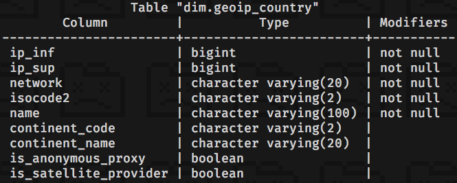
I start from a dim.geoip_country table that is loaded with GeoIP Country CSV downloaded from MaxMind.

Final query
Actually I need only ip_inf, ip_sup and isocode2 fields. The final
query to create the dim.geoip_country_optimized SQL table is the following
INSERT INTO dim.geoip_country_optimized
SELECT
 CASE
  WHEN u.isocode2 = u.prev_isocode2 THEN u.prev_ip_inf
  ELSE u.ip_inf
 END AS ip_inf,
 u.ip_sup,
 u.isocode2
FROM (
 SELECT t.ip_inf, t.ip_sup, t.isocode2,
 LEAD(t.isocode2) OVER (ORDER BY t.ip_inf) AS next_isocode2,
 LAG(t.isocode2) OVER (ORDER BY t.ip_inf) AS prev_isocode2,
 LAG(t.ip_inf) OVER (ORDER BY t.ip_inf) AS prev_ip_inf
 FROM (
  SELECT
   ip_inf,
   ip_sup,
   isocode2,
   LAG(isocode2) OVER (ORDER BY ip_inf) AS prev,
   LEAD(isocode2) OVER (ORDER BY ip_inf) AS next
  FROM dim.geoip_country
 ) t
 WHERE t.isocode2 != t.prev OR t.isocode2 != t.next
) u
WHERE u.isocode2 != u.next_isocode2
;
Step by step
Let’s break it into pieces! I started using LEAD and LAG analytic
functions, with the following query
SELECT
 ip_inf,
 ip_sup,
 isocode2,
 LAG(isocode2) OVER (ORDER BY ip_inf) AS prev,
 LEAD(isocode2) OVER (ORDER BY ip_inf) AS next
FROM dim.geoip_country
ORDER BY 1
to get a result set like
   ip_inf   |   ip_sup   | isocode2 | prev | next
------------+------------+----------+------+------
   16859136 |   16875520 | JP       | CN   | TH
   16875520 |   16908288 | TH       | JP   | CN
   16908288 |   16908800 | CN       | TH   | CN
   16908800 |   16909056 | CN       | CN   | US
   16909056 |   16909312 | US       | CN   | CN
   16909312 |   16910336 | CN       | US   | CN
   16910336 |   16912384 | CN       | CN   | CN
   16912384 |   16916480 | CN       | CN   | CN
   16916480 |   16924672 | CN       | CN   | CN
   16924672 |   16941056 | CN       | CN   | TH
where rows with isocode2 = prev AND isocode2 = next can be discarded.
Using the De Morgan’s laws
to negate this condition and applying this filter a first optimization
is achieved.
SELECT t.ip_inf, t.ip_sup, t.isocode2
FROM (
 SELECT
  ip_inf,
  ip_sup,
  isocode2,
  LAG(isocode2) OVER (ORDER BY ip_inf) AS prev,
  LEAD(isocode2) OVER (ORDER BY ip_inf) AS next
 FROM dim.geoip_country
) t
WHERE t.isocode2 != t.prev OR t.isocode2 != t.next
ORDER BY 1
The result set is the following, so far so good.
   ip_inf   |   ip_sup   | isocode2
------------+------------+----------
   16859136 |   16875520 | JP
   16875520 |   16908288 | TH
   16908288 |   16908800 | CN
   16908800 |   16909056 | CN
   16909056 |   16909312 | US
   16909312 |   16910336 | CN
   16924672 |   16941056 | CN
There are still unnecessary rows, for instance in the result set above,
the ones with CN isocode. Let’s use againg LAG and LEAD to get
the next_isocode2, prev_isocode2 and prev_ip_inf fields.
SELECT
  t.ip_inf, t.ip_sup, t.isocode2,
 LEAD(t.isocode2) OVER (ORDER BY t.ip_inf) AS next_isocode2,
 LAG(t.isocode2) OVER (ORDER BY t.ip_inf) AS prev_isocode2,
 LAG(t.ip_inf) OVER (ORDER BY t.ip_inf) AS prev_ip_inf
FROM (
 SELECT
  ip_inf,
  ip_sup,
  isocode2,
  LAG(isocode2) OVER (ORDER BY ip_inf) AS prev,
  LEAD(isocode2) OVER (ORDER BY ip_inf) AS next
 FROM dim.geoip_country
) t
WHERE t.isocode2 != t.prev OR t.isocode2 != t.next
ORDER BY 1
If you see the result set below you can agree that isocode2 and prev_isocode2
are equal means that there are two consecutive rows with the same country,
for instance CN, hence the first column value desired is prev_ip_inf.
Otherwise it is ok to keep original ip_inf.
This logic is exactly what is implemented in the final query.
   ip_inf   |   ip_sup   | isocode2 | next_isocode2 | prev_isocode2 | prev_ip_inf
------------+------------+----------+---------------+---------------+-------------
   16850944 |   16859136 | CN       | JP            | CN            |    16843264
   16859136 |   16875520 | JP       | TH            | CN            |    16850944
   16875520 |   16908288 | TH       | CN            | JP            |    16859136
   16908288 |   16908800 | CN       | CN            | TH            |    16875520
   16908800 |   16909056 | CN       | US            | CN            |    16908288
   16909056 |   16909312 | US       | CN            | CN            |    16908800
   16909312 |   16910336 | CN       | CN            | US            |    16909056
   16924672 |   16941056 | CN       | TH            | CN            |    16909312